Excel: Highlight Max/Min Values in Rows & Columns!

How to Find the Highest or Lowest Values in Each Rows and Columns using Conditional Formatting in Excel?

Narendhiran Vijayakumar 27 seconds agoLast Updated: June 10, 2025

0 1 2 minutes read

In Excel, highlighting the highest and lowest values in your data can help you quickly spot trends or important figures. This feature is very useful when you’re working with large sets of numbers and want to identify the maximum and minimum values easily. In this tutorial, I’ll show you how to highlight the maximum and minimum values in both rows and columns which makes the data easier to understand and analyze.

Using Conditional Formatting to Highlight Min/Max Values in Rows & Columns:

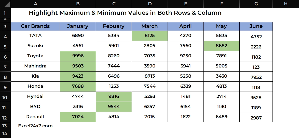
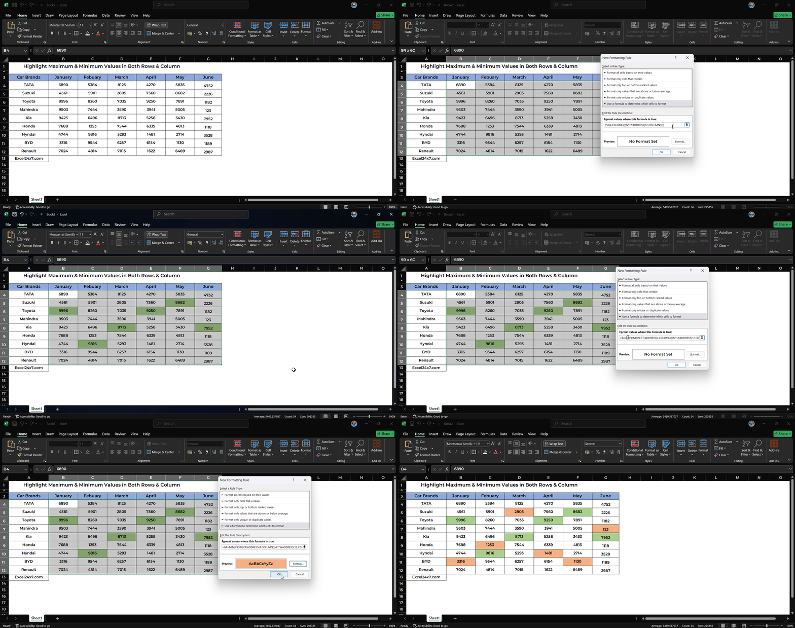
Let me consider a worksheet that contains the sales details of car brands for each month from January to June.

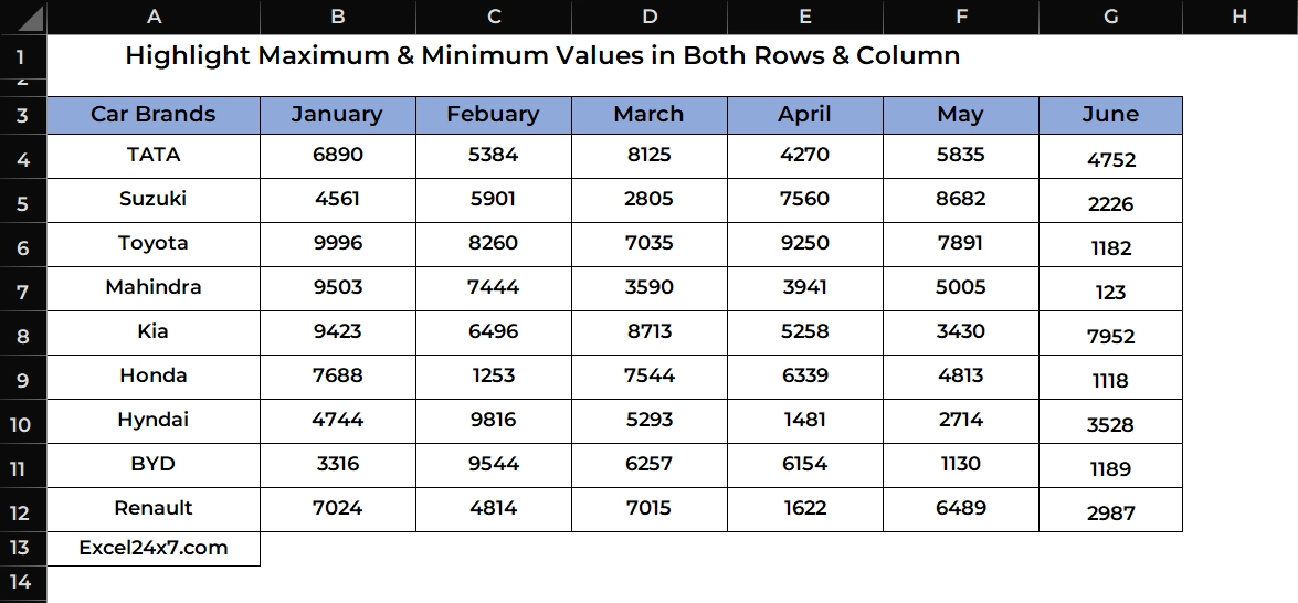
Sample Worksheet of Car Brand Sales Numbers.

Now, I’m going to use the conditional formatting option to find the Maximum & Minimum values for both the rows and column.

Highlight Highest (Maximum) or Lowest (Minimum) values in each row:

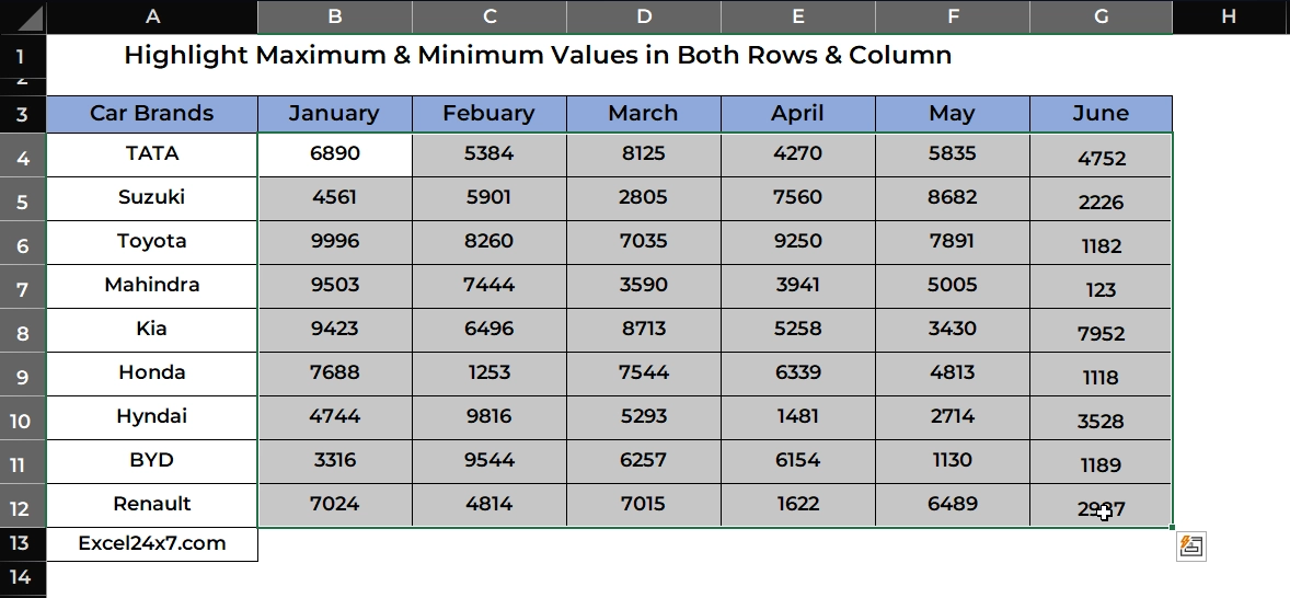
First, you need to choose the range of cells.

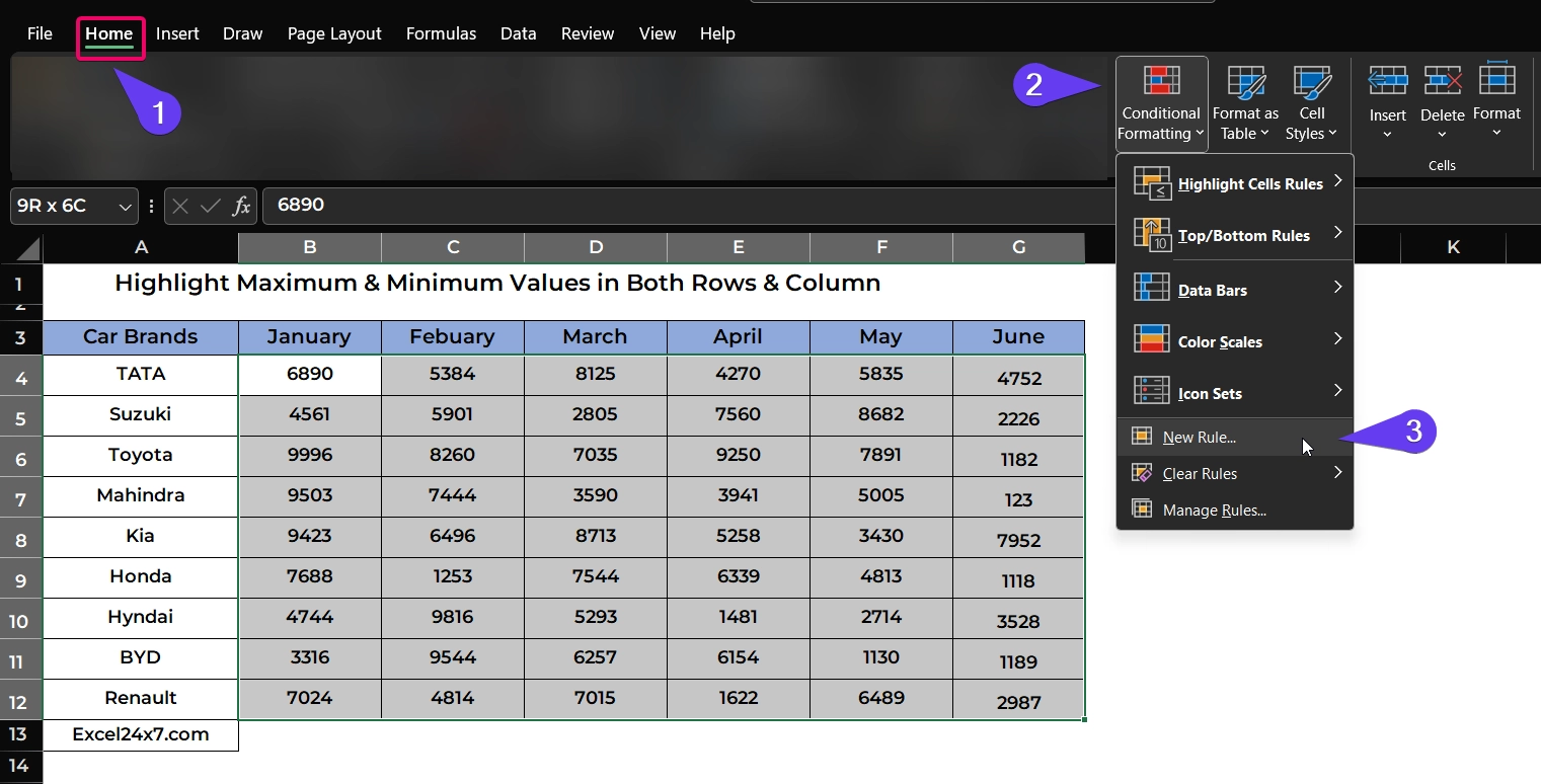
You need to select the range of cell values

In the menu bar, choose the Home -> Conditional Formatting -> New Rules.

Choose conditional formatting and select the New Rules option

Now, in the list, you need to choose the final option “Use a Formula to determine which cells to format” option.
- For highlighting the highest value in each row:
- =B4=MAX($B4:$G4)
- For highlighting the lowest value in each row:
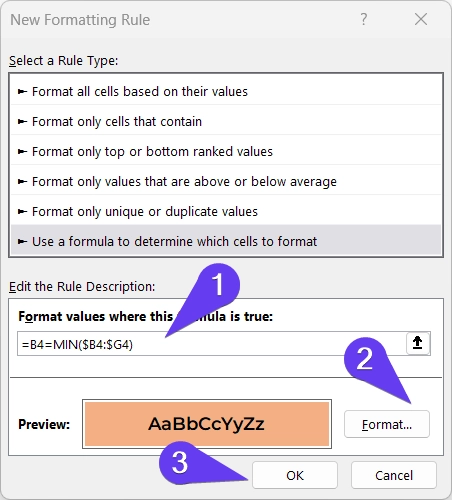
- =B4=MIN($B4:$G4)

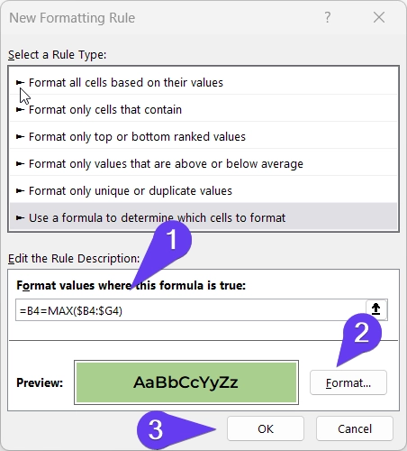
After choosing the formatting options, click the ok button to complete highlighting.

Maximum or Highest Values in Rows has been highlighted.

To highlight the minimum or lowest values, enter the new formula and choose the formatting options and hit the okay button to display the highlighted values.

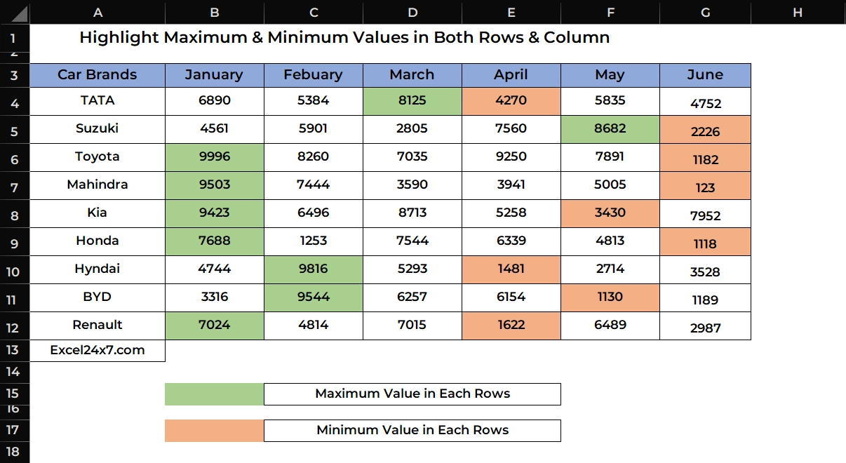
Formatting options for highlighting minimum or lowest values.

Highlighting the Maximum and Minimum Values in the Each Rows using the Conditional Formatting Option.

Highlight Highest (Maximum) or Lowest (Minimum) values in each Column:

First, you need to choose the range of cells.

In the menu bar, choose the Home -> Conditional Formatting -> New Rules.

Now, in the list, you need to choose the final option “Use a Formula to determine which cells to format” option.
- For highlighting the highest value in each column:
- =B4=MAX(INDIRECT(ADDRESS(4,COLUMN())&":"&ADDRESS(12,COLUMN())))
- For highlighting the lowest value in each column:
- =B4=MIN(INDIRECT(ADDRESS(4,COLUMN())&":"&ADDRESS(12,COLUMN())))

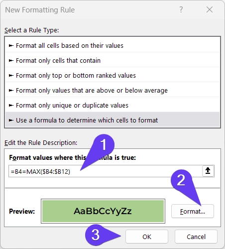
Formatting options to highlight maximum values in each column

Once you’re done, click the ok button to display the highlighted cell values. Repeat the same for highlighting minimum values and click the okay button once you complete formatting options.

Highlighting the Maximum and Minimum Values in the Each Columns using the Conditional Formatting Option.

Functions Used	Used For
MAX	Finds the largest value in a set of numbers.
MIN	Finds the smallest value in a set of numbers.
INDIRECT	Return the reference specified by a text string. Useful for creating dynamic references.
ADDRESS	Create a cell address as a text string, given specified row and column numbers.
COLUMN	Return the column number of a reference.

That’s it.

–Narendhiran Vijayakumar.

Feel free to comment us below, if you have any queries about the above topic and find more interesting excel tutorials on our homepage: Excel24x7.com.